Non-linear interactions

When the interactions between variables contains not only linear terms but also non-linear terms, quadratic for instance, the local field can be written as

\[H_i(t) = \sum_j W_{ij} \sigma_j (t) + \frac{1}{2} \sum_{j,k} Q_{ijk} \sigma_{j}(t) \sigma_{k}(t)\]

The algorithm for inferring couplings \(W_{ij}\) and \(Q_{ijk}\) is similar to the algorithm for inferring only \(W_{ij}\) as described in the Method section. The updated values of couplings are computed as

\[Q_{ijk} = \sum_{\mu, \nu} \langle \delta E_i \delta \sigma_{\mu} \sigma_{\nu} \rangle[C^{-1}]_{j\mu}[C^{-1}]_{k\nu} - \sum_{l} \sum_{\lambda, \mu, \nu} \langle \delta E_i \delta \sigma_l \rangle \langle \delta \sigma_\lambda \delta \sigma_\mu \sigma_\nu \rangle [C^{-1}]_{j\lambda} [C^{-1}]_{k\mu} [C^{-1}]_{l\nu}\]

and

\[W_{ij} = \sum_{k} \lbrace \langle \delta E_i \delta \sigma_k \rangle [C^{-1}]_{kj} - Q_{ijk}\langle \sigma_k \rangle \rbrace\]

In the following, we will demonstrate the performance of our method in inferring the linear couplings \(W_{ij}\) and quadratic couplings \(Q_{ijk}\) from configurations of variables \(\vec \sigma\).

As usual, we start by importing the nesscesary packages into the jupyter notebook.

import numpy as np
import sys
import timeit
import matplotlib.pyplot as plt
import quadratic as quad
%matplotlib inline

np.random.seed(1)

Let us consider a system of n variables. The coupling variability is determined by parameter g.

# parameter setting:
n = 20
g = 1.0

From the parameters, we generate linear couplings \(w_{ij}\) and quadratic couplings \(q_{ijk}\). These are the couplings that our inference algorithms has to reproduce.

w0 = np.random.normal(0.0,g/np.sqrt(n),size=(n,n))
q0 = quad.generate_quadratic(g,n)

Now, from these couplings, we will generate configurations of variables s according to the kinetic Ising model.

l = 5000
s = quad.generate_data(w0,q0,l)

Using the configurations, we will recover the couplings.

w,q = quad.inference(s)

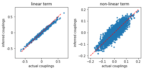
We plot the inferred couplings as function of the actual couplings.

plt.figure(figsize=(6.5,3.2))

plt.subplot2grid((1,2),(0,0))
plt.title('linear term')
plt.plot([-0.6,0.6],[-0.6,0.6],'r--')
plt.scatter(w0,w,s=10)
plt.xlabel('actual couplings')
plt.ylabel('inferred couplings')
plt.xticks([-0.5,0,0.5],('-0.5','0','0.5'))
plt.yticks([-0.5,0,0.5],('-0.5','0','0.5'))
plt.xlim(-0.8,0.8)
plt.ylim(-0.8,0.8)

plt.subplot2grid((1,2),(0,1))
plt.title('non-linear term')
plt.plot([-0.2,0.2],[-0.2,0.2],'r--')
plt.scatter(q0,q,s=10)
plt.xlabel('actual couplings')
plt.ylabel('inferred couplings')

plt.tight_layout(h_pad=1, w_pad=1.5)
plt.show()