Small system

In the following, we will compare the performance of our method, Erasure Machine (EM), with those of other existing methods, including Hopfield approximation (HF), Maximum Likelihood Estimation (MLE), and Pseudo Likelihood Estimations (PLE) (https://github.com/eltrompetero/coniii). We first consider a small system size (e.g., 20 variables) where MLE, PLE are all available. We will see, that in the regime of weak interactions and a large sample size, the EM performs as well as MF, MLE and PLE. However, in the regime of strong interactions and/or a small sample size, EM outperforms MF, MLE and PLE.

We import the necessary packages to the Jupyter notebook:

import matplotlib.pyplot as plt
import numpy as np
import pandas as pd
import emachine as EM

np.random.seed(0)

Weak interactions, and large sample size

We first consider a small system with n_var variables (e.g, n_var = 20) which have weak interactions with each other (e.g., interaction variance parameter g=0.5), and in the limit of a large sample size.

n_var = 20
g = 0.5
n_seq = 800

The synthetic data are generated by using generate_seq.

w_true,seqs = EM.generate_seq(n_var,n_seq,g=g)

For convenience and to reduce computing time (in python), we use Einstein conventions to convert linear and quadratic terms: \(\{ops\} = \{\sigma_i, \sigma_i \sigma_j\}\) (with \(i < j\)). So that, ops is a matrix of n_seq x n_var + 0.5*n_var*(n_var-1).

ops = EM.operators(seqs)

We now reconstruct the interactions from the sequences seqs (or ops).

# Epsilon Machine (EM)
eps_list = np.linspace(0.4,0.9,21)
E_eps = np.zeros(len(eps_list))
w_eps = np.zeros((len(eps_list),ops.shape[1]))
for i,eps in enumerate(eps_list):
    w_eps[i,:],E_eps[i] = EM.fit(ops,eps=eps,max_iter=100)
    #print(eps,E_eps[i])
ieps = np.argmax(E_eps)
print('The optimal value of eps:',eps_list[ieps])

w_em = w_eps[ieps]

The optimal value of eps: 0.75

# Hopfield approximation (HF)
w_hf = EM.hopfield_method(seqs)

# Maximum Likelihood Estimation (MLE)
w_mle = EM.MLE_method(seqs)

# Pseudo Likelihood Estimation (PLE)
w_ple = EM.PLE_method(seqs)

We compare the performance of these methods.

nx,ny = 1,1
fig, ax = plt.subplots(ny,nx,figsize=(nx*3.5,ny*2.8))

ax.plot([-1,1],[-1,1])
ax.plot(w_true,w_hf,'g^',marker='^',mfc='none',markersize=4,label='HF')
ax.plot(w_true,w_mle,'kv',marker='v',mfc='none',markersize=4,label='MLE')
ax.plot(w_true,w_ple,'bs',marker='s',mfc='none',markersize=4,label='PLE')
ax.plot(w_true,w_em,'ro',marker='o',markersize=4,label='EM')
ax.set_xlim([-0.8,0.8])
ax.set_ylim([-0.8,0.8])
ax.set_xticks([-0.8,0,0.8])
ax.set_yticks([-0.8,0,0.8])
ax.set_xlabel('Actual interactions')
ax.set_ylabel('Inferred interactions')

ax.legend()

<matplotlib.legend.Legend at 0x7fd04853e668>

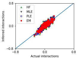
Mean squared error between actuall and inferred interactions of these methods:

MSE_em = ((w_true - w_em)**2).mean()
MSE_hf = ((w_true - w_hf)**2).mean()
MSE_mle = ((w_true - w_mle)**2).mean()
MSE_ple = ((w_true - w_ple)**2).mean()

df = pd.DataFrame([['EM',MSE_em],['HF',MSE_hf],['MLE',MSE_mle],['PLE',MSE_ple]],
                  columns = ['Method','Mean squared error'])
df

	Method	Mean squared error
0	EM	0.002628
1	HF	0.004474
2	MLE	0.002442
3	PLE	0.002715

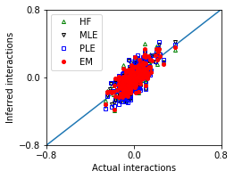
Weak interactions, and small sample size

n_var = 20
g = 0.5
n_seq = 200

w_true,seqs = EM.generate_seq(n_var,n_seq,g=g)

ops = EM.operators(seqs)
eps_list = np.linspace(0.4,0.9,21)
E_eps = np.zeros(len(eps_list))
w_eps = np.zeros((len(eps_list),ops.shape[1]))
for i,eps in enumerate(eps_list):
    w_eps[i,:],E_eps[i] = EM.fit(ops,eps=eps,max_iter=100)
    #print(eps,E_eps[i])
ieps = np.argmax(E_eps)
print('The optimal value of eps:',eps_list[ieps])

w_em = w_eps[ieps]

w_hf = EM.hopfield_method(seqs)
w_mle = EM.MLE_method(seqs)
w_ple = EM.PLE_method(seqs)

The optimal value of eps: 0.775

nx,ny = 1,1
fig, ax = plt.subplots(ny,nx,figsize=(nx*3.5,ny*2.8))

ax.plot([-1,1],[-1,1])
ax.plot(w_true,w_hf,'g^',marker='^',mfc='none',markersize=4,label='HF')
ax.plot(w_true,w_mle,'kv',marker='v',mfc='none',markersize=4,label='MLE')
ax.plot(w_true,w_ple,'bs',marker='s',mfc='none',markersize=4,label='PLE')
ax.plot(w_true,w_em,'ro',marker='o',markersize=4,label='EM')
ax.set_xlim([-0.8,0.8])
ax.set_ylim([-0.8,0.8])
ax.set_xticks([-0.8,0,0.8])
ax.set_yticks([-0.8,0,0.8])
ax.set_xlabel('Actual interactions')
ax.set_ylabel('Inferred interactions')

ax.legend()

<matplotlib.legend.Legend at 0x7fd04836f400>

MSE_em = ((w_true - w_em)**2).mean()
MSE_hf = ((w_true - w_hf)**2).mean()
MSE_mle = ((w_true - w_mle)**2).mean()
MSE_ple = ((w_true - w_ple)**2).mean()

df = pd.DataFrame([['EM',MSE_em],['HF',MSE_hf],['MLE',MSE_mle],['PLE',MSE_ple]],
                  columns = ['Method','Mean squared error'])
df

	Method	Mean squared error
0	EM	0.007569
1	HF	0.008781
2	MLE	0.008984
3	PLE	0.011128

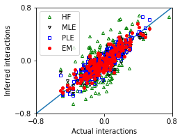
Strong interactions and large sample size

n_var = 20
g = 1.0
n_seq = 1000

w_true,seqs = EM.generate_seq(n_var,n_seq,g=g)

ops = EM.operators(seqs)
eps_list = np.linspace(0.4,0.9,21)
E_eps = np.zeros(len(eps_list))
w_eps = np.zeros((len(eps_list),ops.shape[1]))
for i,eps in enumerate(eps_list):
    w_eps[i,:],E_eps[i] = EM.fit(ops,eps=eps,max_iter=100)
    #print(eps,E_eps[i])
ieps = np.argmax(E_eps)
print('The optimal value of eps:',eps_list[ieps])

w_em = w_eps[ieps]

w_hf = EM.hopfield_method(seqs)
w_mle = EM.MLE_method(seqs)
w_ple = EM.PLE_method(seqs)

The optimal value of eps: 0.65

nx,ny = 1,1
fig, ax = plt.subplots(ny,nx,figsize=(nx*3.5,ny*2.8))

ax.plot([-1,1],[-1,1])
ax.plot(w_true,w_hf,'g^',marker='^',mfc='none',markersize=4,label='HF')
ax.plot(w_true,w_mle,'kv',marker='v',mfc='none',markersize=4,label='MLE')
ax.plot(w_true,w_ple,'bs',marker='s',mfc='none',markersize=4,label='PLE')
ax.plot(w_true,w_em,'ro',marker='o',markersize=4,label='EM')
ax.set_xlim([-0.8,0.8])
ax.set_ylim([-0.8,0.8])
ax.set_xticks([-0.8,0,0.8])
ax.set_yticks([-0.8,0,0.8])
ax.set_xlabel('Actual interactions')
ax.set_ylabel('Inferred interactions')

ax.legend()

<matplotlib.legend.Legend at 0x7fd04a6859b0>

MSE_em = ((w_true - w_em)**2).mean()
MSE_hf = ((w_true - w_hf)**2).mean()
MSE_mle = ((w_true - w_mle)**2).mean()
MSE_ple = ((w_true - w_ple)**2).mean()

df = pd.DataFrame([['EM',MSE_em],['HF',MSE_hf],['MLE',MSE_mle],['PLE',MSE_ple]],
                  columns = ['Method','Mean squared error'])
df

	Method	Mean squared error
0	EM	0.008664
1	HF	0.041372
2	MLE	0.010525
3	PLE	0.008515

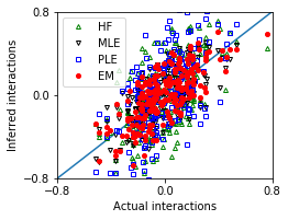
Strong interactions and small sample size

n_var = 20
g = 1.0
n_seq = 200

w_true,seqs = EM.generate_seq(n_var,n_seq,g=g)

ops = EM.operators(seqs)
eps_list = np.linspace(0.4,0.9,21)
E_eps = np.zeros(len(eps_list))
w_eps = np.zeros((len(eps_list),ops.shape[1]))
for i,eps in enumerate(eps_list):
    w_eps[i,:],E_eps[i] = EM.fit(ops,eps=eps,max_iter=100)
    #print(eps,E_eps[i])
ieps = np.argmax(E_eps)
print('The optimal value of eps:',eps_list[ieps])

w_em = w_eps[ieps]

w_hf = EM.hopfield_method(seqs)
w_mle = EM.MLE_method(seqs)
w_ple = EM.PLE_method(seqs)

The optimal value of eps: 0.7250000000000001

nx,ny = 1,1
fig, ax = plt.subplots(ny,nx,figsize=(nx*3.5,ny*2.8))

ax.plot([-1,1],[-1,1])
ax.plot(w_true,w_hf,'g^',marker='^',mfc='none',markersize=4,label='HF')
ax.plot(w_true,w_mle,'kv',marker='v',mfc='none',markersize=4,label='MLE')
ax.plot(w_true,w_ple,'bs',marker='s',mfc='none',markersize=4,label='PLE')
ax.plot(w_true,w_em,'ro',marker='o',markersize=4,label='EM')
ax.set_xlim([-0.8,0.8])
ax.set_ylim([-0.8,0.8])
ax.set_xticks([-0.8,0,0.8])
ax.set_yticks([-0.8,0,0.8])
ax.set_xlabel('Actual interactions')
ax.set_ylabel('Inferred interactions')

ax.legend()

<matplotlib.legend.Legend at 0x7fd04a8563c8>

MSE_em = ((w_true - w_em)**2).mean()
MSE_hf = ((w_true - w_hf)**2).mean()
MSE_mle = ((w_true - w_mle)**2).mean()
MSE_ple = ((w_true - w_ple)**2).mean()

df = pd.DataFrame([['EM',MSE_em],['HF',MSE_hf],['MLE',MSE_mle],['PLE',MSE_ple]],
                  columns = ['Method','Mean squared error'])
df

	Method	Mean squared error
0	EM	0.029413
1	HF	0.079308
2	MLE	0.034116
3	PLE	0.095591