Large system
We now consider a larger system (e.g., 40 variables). MLE is intractable. Thus, we can just compare the performance of EM with HF and PLE.
As usual, we import the necessary packages to the Jupyter notebook:
[1]:
import matplotlib.pyplot as plt
import numpy as np
import pandas as pd
import emachine as EM
[2]:
np.random.seed(0)
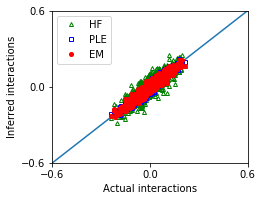
Weak interactions and large sample size
[3]:
n_var = 40
g = 0.5
n_seq = 8000
The synthetic data are generated by using generate_seq.
[4]:
w_true,seqs = EM.generate_seq(n_var,n_seq,g=g)
We reconstruct the interactions from the sequences seqs (or ops).
[5]:
# Erasure Machine (EM)
ops = EM.operators(seqs)
eps_list = np.linspace(0.5,0.8,16)
E_eps = np.zeros(len(eps_list))
w_eps = np.zeros((len(eps_list),ops.shape[1]))
for i,eps in enumerate(eps_list):
    w_eps[i,:],E_eps[i] = EM.fit(ops,eps=eps,max_iter=100)
    #print(eps,E_eps[i])
ieps = np.argmax(E_eps)
print('The optimal value of eps:',eps_list[ieps])

w_em = w_eps[ieps]
The optimal value of eps: 0.64
[6]:
# Hopfield approximation (HF)
w_hf = EM.hopfield_method(seqs)

# Pseudo Likelihood Estimation (PLE)
w_ple = EM.PLE_method(seqs)
We compare the performances of these methods.
[7]:
nx,ny = 1,1
fig, ax = plt.subplots(ny,nx,figsize=(nx*3.5,ny*2.8))

ax.plot([-1,1],[-1,1])
ax.plot(w_true,w_hf,'g^',marker='^',mfc='none',markersize=4,label='HF')
ax.plot(w_true,w_ple,'bs',marker='s',mfc='none',markersize=4,label='PLE')
ax.plot(w_true,w_em,'ro',marker='o',markersize=4,label='EM')
ax.set_xlim([-0.6,0.6])
ax.set_ylim([-0.6,0.6])
ax.set_xticks([-0.6,0,0.6])
ax.set_yticks([-0.6,0,0.6])
ax.set_xlabel('Actual interactions')
ax.set_ylabel('Inferred interactions')

ax.legend()
[7]:
<matplotlib.legend.Legend at 0x7fd16f694a58>
[8]:
MSE_em = ((w_true - w_em)**2).mean()
MSE_hf = ((w_true - w_hf)**2).mean()
MSE_ple = ((w_true - w_ple)**2).mean()

df = pd.DataFrame([['EM',MSE_em],['HF',MSE_hf],['PLE',MSE_ple]],
                  columns = ['Method','Mean squared error'])
df
[8]:
| Method | Mean squared error | |
|---|---|---|
| 0 | EM | 0.000515 |
| 1 | HF | 0.002071 |
| 2 | PLE | 0.000494 |
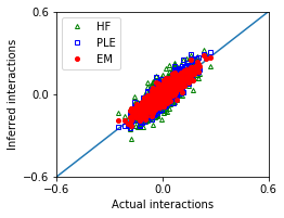
Weak interactions, and small sample size
[9]:
n_var = 40
g = 0.5
n_seq = 2000
[10]:
w_true,seqs = EM.generate_seq(n_var,n_seq,g=g)
[11]:
ops = EM.operators(seqs)
eps_list = np.linspace(0.5,0.8,16)
E_eps = np.zeros(len(eps_list))
w_eps = np.zeros((len(eps_list),ops.shape[1]))
for i,eps in enumerate(eps_list):
    w_eps[i,:],E_eps[i] = EM.fit(ops,eps=eps,max_iter=100)
    #print(eps,E_eps[i])
ieps = np.argmax(E_eps)
print('The optimal value of eps:',eps_list[ieps])

w_em = w_eps[ieps]

w_hf = EM.hopfield_method(seqs)
w_ple = EM.PLE_method(seqs)
The optimal value of eps: 0.72
[12]:
nx,ny = 1,1
fig, ax = plt.subplots(ny,nx,figsize=(nx*3.5,ny*2.8))

ax.plot([-1,1],[-1,1])
ax.plot(w_true,w_hf,'g^',marker='^',mfc='none',markersize=4,label='HF')
ax.plot(w_true,w_ple,'bs',marker='s',mfc='none',markersize=4,label='PLE')
ax.plot(w_true,w_em,'ro',marker='o',markersize=4,label='EM')
ax.set_xlim([-0.6,0.6])
ax.set_ylim([-0.6,0.6])
ax.set_xticks([-0.6,0,0.6])
ax.set_yticks([-0.6,0,0.6])
ax.set_xlabel('Actual interactions')
ax.set_ylabel('Inferred interactions')

ax.legend()
[12]:
<matplotlib.legend.Legend at 0x7fd170168b70>
[13]:
MSE_em = ((w_true - w_em)**2).mean()
MSE_hf = ((w_true - w_hf)**2).mean()
MSE_ple = ((w_true - w_ple)**2).mean()

df = pd.DataFrame([['EM',MSE_em],['HF',MSE_hf],['PLE',MSE_ple]],
                  columns = ['Method','Mean squared error'])
df
[13]:
| Method | Mean squared error | |
|---|---|---|
| 0 | EM | 0.001388 |
| 1 | HF | 0.003787 |
| 2 | PLE | 0.002020 |
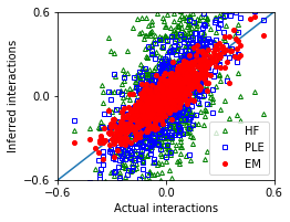
Strong interactions and large sample size
[14]:
n_var = 40
g = 1.0
n_seq = 8000
[15]:
w_true,seqs = EM.generate_seq(n_var,n_seq,g=g)
[16]:
ops = EM.operators(seqs)
eps_list = np.linspace(0.5,0.8,16)
E_eps = np.zeros(len(eps_list))
w_eps = np.zeros((len(eps_list),ops.shape[1]))
for i,eps in enumerate(eps_list):
    w_eps[i,:],E_eps[i] = EM.fit(ops,eps=eps,max_iter=100)
    #print(eps,E_eps[i])
ieps = np.argmax(E_eps)
print('The optimal value of eps:',eps_list[ieps])

w_em = w_eps[ieps]

w_hf = EM.hopfield_method(seqs)
w_ple = EM.PLE_method(seqs)
The optimal value of eps: 0.64
[17]:
nx,ny = 1,1
fig, ax = plt.subplots(ny,nx,figsize=(nx*3.5,ny*2.8))

ax.plot([-1,1],[-1,1])
ax.plot(w_true,w_hf,'g^',marker='^',mfc='none',markersize=4,label='HF')
ax.plot(w_true,w_ple,'bs',marker='s',mfc='none',markersize=4,label='PLE')
ax.plot(w_true,w_em,'ro',marker='o',markersize=4,label='EM')
ax.set_xlim([-0.6,0.6])
ax.set_ylim([-0.6,0.6])
ax.set_xticks([-0.6,0,0.6])
ax.set_yticks([-0.6,0,0.6])
ax.set_xlabel('Actual interactions')
ax.set_ylabel('Inferred interactions')

ax.legend()
[17]:
<matplotlib.legend.Legend at 0x7fd16fbbef60>
[18]:
MSE_em = ((w_true - w_em)**2).mean()
MSE_hf = ((w_true - w_hf)**2).mean()
MSE_ple = ((w_true - w_ple)**2).mean()

df = pd.DataFrame([['EM',MSE_em],['HF',MSE_hf],['PLE',MSE_ple]],
                  columns = ['Method','Mean squared error'])
df
[18]:
| Method | Mean squared error | |
|---|---|---|
| 0 | EM | 0.005574 |
| 1 | HF | 0.077182 |
| 2 | PLE | 0.029280 |
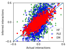
Strong interactions and small sample size
[19]:
n_var = 40
g = 1.0
n_seq = 2000
[20]:
w_true,seqs = EM.generate_seq(n_var,n_seq,g=g)
[21]:
ops = EM.operators(seqs)
eps_list = np.linspace(0.5,0.8,16)
E_eps = np.zeros(len(eps_list))
w_eps = np.zeros((len(eps_list),ops.shape[1]))
for i,eps in enumerate(eps_list):
    w_eps[i,:],E_eps[i] = EM.fit(ops,eps=eps,max_iter=100)
    #print(eps,E_eps[i])
ieps = np.argmax(E_eps)
print('The optimal value of eps:',eps_list[ieps])
w_em = w_eps[ieps]

print('Hopfield')
w_hf = EM.hopfield_method(seqs)

print('PLE')
w_ple = EM.PLE_method(seqs)
The optimal value of eps: 0.68
Hopfield
PLE
[22]:
nx,ny = 1,1
fig, ax = plt.subplots(ny,nx,figsize=(nx*3.5,ny*2.8))

ax.plot([-1,1],[-1,1])
ax.plot(w_true,w_hf,'g^',marker='^',mfc='none',markersize=4,label='HF')
ax.plot(w_true,w_ple,'bs',marker='s',mfc='none',markersize=4,label='PLE')
ax.plot(w_true,w_em,'ro',marker='o',markersize=4,label='EM')
ax.set_xlim([-0.6,0.6])
ax.set_ylim([-0.6,0.6])
ax.set_xticks([-0.6,0,0.6])
ax.set_yticks([-0.6,0,0.6])
ax.set_xlabel('Actual interactions')
ax.set_ylabel('Inferred interactions')

ax.legend()
[22]:
<matplotlib.legend.Legend at 0x7fd16fd23198>
[23]:
MSE_em = ((w_true - w_em)**2).mean()
MSE_hf = ((w_true - w_hf)**2).mean()
MSE_ple = ((w_true - w_ple)**2).mean()

df = pd.DataFrame([['EM',MSE_em],['HF',MSE_hf],['PLE',MSE_ple]],
                  columns = ['Method','Mean squared error'])
df
[23]:
| Method | Mean squared error | |
|---|---|---|
| 0 | EM | 0.009827 |
| 1 | HF | 0.079888 |
| 2 | PLE | 0.061577 |
[ ]: