Very large system
We now consider a very large system (e.g., 100 variables). PLE is intractable, thus only EM and HF can work for such large systems. We will see that EM works better than HF in every case that we consider.
[1]:
import matplotlib.pyplot as plt
import numpy as np
import pandas as pd
import emachine as EM
[2]:
np.random.seed(0)
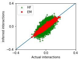
Weak interactions and large sample size
[3]:
n_var = 100
g = 0.5
n_seq = 40000
The synthetic data are generated by using generate_seq.
[4]:
w_true,seqs = EM.generate_seq(n_var,n_seq,g=g)
We reconstruct the interactions from the sequences seqs (or ops).
[5]:
# Erasure Machine (EM)
ops = EM.operators(seqs)
eps_list = np.linspace(0.4,0.8,5)
E_eps = np.zeros(len(eps_list))
w_eps = np.zeros((len(eps_list),ops.shape[1]))
for i,eps in enumerate(eps_list):
    w_eps[i,:],E_eps[i] = EM.fit(ops,eps=eps,max_iter=100)
    #print(eps,E_eps[i])
ieps = np.argmax(E_eps)
print('The optimal value of eps:',eps_list[ieps])

w_em = w_eps[ieps]

# Hopfield approximation (HF)
w_hf = EM.hopfield_method(seqs)
The optimal value of eps: 0.7000000000000001
We compare the performance of these methods.
[6]:
nx,ny = 1,1
fig, ax = plt.subplots(ny,nx,figsize=(nx*3.5,ny*2.8))

ax.plot([-1,1],[-1,1])
ax.plot(w_true,w_hf,'g^',marker='^',mfc='none',markersize=4,label='HF')
ax.plot(w_true,w_em,'ro',marker='o',markersize=4,label='EM')
ax.set_xlim([-0.4,0.4])
ax.set_ylim([-0.4,0.4])
ax.set_xticks([-0.4,0,0.4])
ax.set_yticks([-0.4,0,0.4])
ax.set_xlabel('Actual interactions')
ax.set_ylabel('Inferred interactions')

ax.legend()
[6]:
<matplotlib.legend.Legend at 0x7fc9847863c8>
[7]:
MSE_em = ((w_true - w_em)**2).mean()
MSE_hf = ((w_true - w_hf)**2).mean()

df = pd.DataFrame([['EM',MSE_em],['HF',MSE_hf]],
                  columns = ['Method','Mean squared error'])
df
[7]:
| Method | Mean squared error | |
|---|---|---|
| 0 | EM | 0.000249 |
| 1 | HF | 0.002642 |
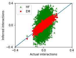
Weak interactions, and small sample size
[8]:
n_var = 100
g = 0.5
n_seq = 10000
[9]:
w_true,seqs = EM.generate_seq(n_var,n_seq,g=g)
[10]:
ops = EM.operators(seqs)
eps_list = np.linspace(0.4,0.8,5)
E_eps = np.zeros(len(eps_list))
w_eps = np.zeros((len(eps_list),ops.shape[1]))
for i,eps in enumerate(eps_list):
    w_eps[i,:],E_eps[i] = EM.fit(ops,eps=eps,max_iter=100)
    #print(eps,E_eps[i])
ieps = np.argmax(E_eps)
print('The optimal value of eps:',eps_list[ieps])

w_em = w_eps[ieps]

w_hf = EM.hopfield_method(seqs)
The optimal value of eps: 0.7000000000000001
[11]:
nx,ny = 1,1
fig, ax = plt.subplots(ny,nx,figsize=(nx*3.5,ny*2.8))

ax.plot([-1,1],[-1,1])
ax.plot(w_true,w_hf,'g^',marker='^',mfc='none',markersize=4,label='HF')
ax.plot(w_true,w_em,'ro',marker='o',markersize=4,label='EM')
ax.set_xlim([-0.4,0.4])
ax.set_ylim([-0.4,0.4])
ax.set_xticks([-0.4,0,0.4])
ax.set_yticks([-0.4,0,0.4])
ax.set_xlabel('Actual interactions')
ax.set_ylabel('Inferred interactions')

ax.legend()
[11]:
<matplotlib.legend.Legend at 0x7fc98466e0f0>
[12]:
MSE_em = ((w_true - w_em)**2).mean()
MSE_hf = ((w_true - w_hf)**2).mean()

df = pd.DataFrame([['EM',MSE_em],['HF',MSE_hf]],
                  columns = ['Method','Mean squared error'])
df
[12]:
| Method | Mean squared error | |
|---|---|---|
| 0 | EM | 0.000763 |
| 1 | HF | 0.016874 |
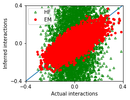
Strong interactions
[13]:
n_var = 100
g = 1.0
n_seq = 40000
[14]:
w_true,seqs = EM.generate_seq(n_var,n_seq,g=g)
[15]:
ops = EM.operators(seqs)
eps_list = np.linspace(0.4,0.8,5)
E_eps = np.zeros(len(eps_list))
w_eps = np.zeros((len(eps_list),ops.shape[1]))
for i,eps in enumerate(eps_list):
    w_eps[i,:],E_eps[i] = EM.fit(ops,eps=eps,max_iter=100)
    #print(eps,E_eps[i])
ieps = np.argmax(E_eps)
print('The optimal value of eps:',eps_list[ieps])

w_em = w_eps[ieps]

w_hf = EM.hopfield_method(seqs)
The optimal value of eps: 0.7000000000000001
[16]:
nx,ny = 1,1
fig, ax = plt.subplots(ny,nx,figsize=(nx*3.5,ny*2.8))

ax.plot([-1,1],[-1,1])
ax.plot(w_true,w_hf,'g^',marker='^',mfc='none',markersize=4,label='HF')
ax.plot(w_true,w_em,'ro',marker='o',markersize=4,label='EM')
ax.set_xlim([-0.4,0.4])
ax.set_ylim([-0.4,0.4])
ax.set_xticks([-0.4,0,0.4])
ax.set_yticks([-0.4,0,0.4])
ax.set_xlabel('Actual interactions')
ax.set_ylabel('Inferred interactions')

ax.legend()
[16]:
<matplotlib.legend.Legend at 0x7fc9846467f0>
[17]:
MSE_em = ((w_true - w_em)**2).mean()
MSE_hf = ((w_true - w_hf)**2).mean()

df = pd.DataFrame([['EM',MSE_em],['HF',MSE_hf]],
                  columns = ['Method','Mean squared error'])
df
[17]:
| Method | Mean squared error | |
|---|---|---|
| 0 | EM | 0.005028 |
| 1 | HF | 0.083528 |