Comparison: MLE vs. FEM

As shown in the previous sections, it is clear that mean field approximations such as nMF, TAP, and eMF do not perform as well as MLE and FEM. In the following, we therefore focus only MLE and FEM. We demonstrate that FEM works as well as MLE in the small coupling variability regime but FEM outperforms MLE in the difficult large coupling variability regime.

Beside better performance, FEM has some computational merits. First, FEM parameter updates are multiplicative while MLE updates are computed by trying to maximize a likelihood function, usually by gradient ascent or variants. In our hands, without special code tuning for either algorithm, FEM works faster than MLE. Second, MLE has a learning rate parameter while FEM does not have any tunable parameter.

As usual, first of all, the necessary packages are imported to the jupyter notebook.

import numpy as np
import sys
import timeit
import matplotlib.pyplot as plt
import simulate
import inference
%matplotlib inline

np.random.seed(1)

We consider a system of \(N = 100\) variables and \(L=2000\) datapoints for the demonstrations below. A learning rate rate \(= 1\) is selected for MLE.

# parameter setting:
n = 100
l = 2000
rate = 1.

Small coupling variability

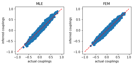
We first consider the small coupling variability regime, g = 2.0.

g = 2.0

We generate a random coupling matrix:

w0 = np.random.normal(0.0,g/np.sqrt(n),size=(n,n))

The configurations of variables are also generated:

s = simulate.generate_data(w0,l)

We now apply MLE to recover the coupling matrix w0 from the configurations s. As shown in the MLE section, the performance of MLE can be improved by using our stopping criterion. Additionally, our stopping criterion can help MLE avoid unnecessary iterations. As a concrete illustration, in the following, we consider MLE with our stopping criterion. We can select this option by setting stop_criterion='yes'.

print('MLE:')
start_time = timeit.default_timer()

wMLE = inference.mle(s,rate,stop_criterion='yes')

stop_time=timeit.default_timer()
run_time=stop_time-start_time
print('run_time:',run_time)

MSE_MLE = np.mean((wMLE-w0)**2)
print('MSE:',MSE_MLE)

MLE:
('run_time:', 9.159331798553467)
('MSE:', 0.0029889738951087916)

For comparison, we also apply FEM to recover the coupling matrix.

print('FEM:')
start_time = timeit.default_timer()

wFEM = inference.fem(s)

stop_time=timeit.default_timer()
run_time=stop_time-start_time
print('run_time:',run_time)

MSE_FEM = np.mean((wFEM-w0)**2)
print('MSE:',MSE_FEM)

FEM:
('run_time:', 0.4248168468475342)
('MSE:', 0.002227111736127038)

The result shows that the mean square error (MSE) obtaining from FEM is slighty lower than that from MLE. Additionally, FEM works faster than MLE.

The inferred couplings are plotted as function of actual couplings:

plt.figure(figsize=(6.5,3.2))

plt.subplot2grid((1,2),(0,0))
plt.title('MLE')
plt.plot([-1,1],[-1,1],'r--')
plt.scatter(w0,wMLE)
plt.xlabel('actual couplings')
plt.ylabel('inferred couplings')

plt.subplot2grid((1,2),(0,1))
plt.title('FEM')
plt.plot([-1,1],[-1,1],'r--')
plt.scatter(w0,wFEM)
plt.xlabel('actual couplings')
plt.ylabel('inferred couplings')

plt.tight_layout(h_pad=1, w_pad=1.5)
plt.show()

Large coupling variability

Now, we consider the difficult regime (large coupling variability): g = 4.0.

g = 4.0

As above, a coupling matrix w0 is generated. From these couplings, we generate configurations of variables s.

w0 = np.random.normal(0.0,g/np.sqrt(n),size=(n,n))
s = simulate.generate_data(w0,l)

We first use MLE to recover the coupling matrix from the configurations:

print('MLE:')
start_time = timeit.default_timer()

wMLE = inference.mle(s,rate,stop_criterion='yes')

stop_time=timeit.default_timer()
run_time=stop_time-start_time
print('run_time:',run_time)

MSE_MLE = np.mean((wMLE-w0)**2)
print('MSE:',MSE_MLE)

MLE:
('run_time:', 81.38691401481628)
('MSE:', 0.0172333170396427)

FEM is also used to recover the coupling matrix:

print('FEM:')
start_time = timeit.default_timer()

wFEM = inference.fem(s)

stop_time=timeit.default_timer()
run_time=stop_time-start_time
print('run_time:',run_time)

MSE_FEM = np.mean((wFEM-w0)**2)
print('MSE:',MSE_FEM)

FEM:
('run_time:', 1.8361680507659912)
('MSE:', 0.006308420614357616)

plt.figure(figsize=(6.5,3.2))

plt.subplot2grid((1,2),(0,0))
plt.title('MLE')
plt.plot([-2.,2.],[-2.0,2.0],'r--')
plt.scatter(w0,wMLE)
plt.xlabel('actual couplings')
plt.ylabel('inferred couplings')

plt.subplot2grid((1,2),(0,1))
plt.title('FEM')
plt.plot([-2.,2.],[-2.0,2.0],'r--')
plt.scatter(w0,wFEM)
plt.xlabel('actual couplings')
plt.ylabel('inferred couplings')

plt.tight_layout(h_pad=1, w_pad=1.5)
plt.show()

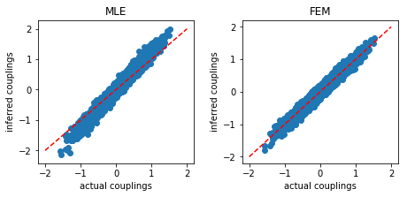
These results show that the MSE obtained using FEM is significantly lower than MLE, and FEM works much faster than MLE, even when MLE is used with our stopping criterion to speed it up.