Maximum Likelihood Estimation
![]()
Maximum likelihood estimation (MLE) is a standard method in the field of network inference. The MLE algorithm for the kinetic Ising model contains the following steps:
Initialize \(W_{ij}\) at random;
Compute the local field \(H_i(t) = \sum_j W_{ij} \sigma_j (t)\);
Compute the probability;
\[P[\sigma_i(t+1)|\vec{\sigma}(t)] = \frac{\exp [ \sigma_i(t+1) H_i(t)]}{\sum_{\sigma_i(t+1)} \exp[\sigma_i(t+1) H_i(t)]}\]Compute the likelihood \(\mathcal{P}_i = \prod_{t=1}^{L-1}P[\sigma_i(t+1)|\vec{\sigma}(t)]\);
Update \(W_{ij}\) through \(W_{ij}^{\textrm{new}} = W_{ij} + \frac{\alpha}{L-1} \frac{\partial \log {\cal{P}}_i }{\partial W_{ij}}\) where \(\alpha\) is a learning rate parameter, and \(\frac{\partial \log {\mathcal{P}}_i}{\partial W_{ij}} = \sum_{t=1}^{L-1} \lbrace \sigma_i(t+1) \sigma_j(t) - \tanh [H_i(t)] \sigma_j(t) \rbrace\);
Repeat steps (ii)-(v);
Perform (ii)-(vi) in parallel for every variable index \(i \in \{1, 2, \cdots, N\}\).
In the following, we will test the performance of this method for various cases: small coupling variability and large coupling variability. We will show that MLE starts to overfit in the regime of large coupling variability and small sample sizes. Applying our stopping criterion to MLE can make this method works significantly faster and somewhat more accurately.
First of all, we import some packages to the jupyter notebook:
In [1]:
import numpy as np
import sys
import timeit
import matplotlib.pyplot as plt
import simulate
import inference
%matplotlib inline

np.random.seed(1)
We first consider a system of \(N = 100\) variables. Data length \(L=2000\) is used for this illustration with a learning rate \(\alpha=1.\)
In [2]:
# parameter setting:
n = 100
l = 2000
rate = 1.
Small coupling variability \((g = 2)\)
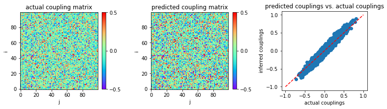
For the regime of small coupling variability, as with the other methods, we select \(g = 2.0\) for the demonstration.
In [3]:
g = 2.0
The actual coupling matrix is generated as follows:
In [4]:
w0 = np.random.normal(0.0,g/np.sqrt(n),size=(n,n))
From the coupling matrix, we generate a time series of variables based on the kinetic Ising model:
In [5]:
s = simulate.generate_data(w0,l)
Without our stopping criterion
Similar to FEM and eMF, MLE is an iterative algorithm. We first run this method as described in the literature, without a stopping criterion.
In [6]:
start_time = timeit.default_timer()

w = inference.mle(s,rate,stop_criterion='no')

stop_time=timeit.default_timer()
run_time=stop_time-start_time
print('run_time:',run_time)
('run_time:', 158.09815406799316)
The inferred couplings are plotted to compare with actual couplings:
In [7]:
plt.figure(figsize=(11,3.2))

plt.subplot2grid((1,3),(0,0))
plt.title('actual coupling matrix')
plt.imshow(w0,cmap='rainbow',origin='lower')
plt.xlabel('j')
plt.ylabel('i')
plt.clim(-0.5,0.5)
plt.colorbar(fraction=0.045, pad=0.05,ticks=[-0.5,0,0.5])

plt.subplot2grid((1,3),(0,1))
plt.title('predicted coupling matrix')
plt.imshow(w,cmap='rainbow',origin='lower')
plt.xlabel('j')
plt.ylabel('i')
plt.clim(-0.5,0.5)
plt.colorbar(fraction=0.045, pad=0.05,ticks=[-0.5,0,0.5])

plt.subplot2grid((1,3),(0,2))
plt.title('predicted couplings vs. actual couplings')
plt.plot([-1,1],[-1,1],'r--')
plt.scatter(w0,w)
plt.xlabel('actual couplings')
plt.ylabel('inferred couplings')

plt.tight_layout(h_pad=1, w_pad=1.5)
plt.show()

Mean square error is calculated as the following:
In [8]:
MSE = np.mean((w-w0)**2)
print('MSE:',MSE)
('MSE:', 0.0030760425560816744)
With our stopping criterion
Now, we apply our stopping criterion for this method. According to this criterion, we stop the iteration when the discrepancy between observed variables and its model expectations starts to increase.
In [9]:
start_time = timeit.default_timer()

w = inference.mle(s,rate,stop_criterion='yes')

stop_time=timeit.default_timer()
run_time=stop_time-start_time
print('run_time:',run_time)
('run_time:', 8.734601020812988)
The inferred couplings are plotted:
In [10]:
plt.figure(figsize=(11,3.2))

plt.subplot2grid((1,3),(0,0))
plt.title('actual coupling matrix')
plt.imshow(w0,cmap='rainbow',origin='lower')
plt.xlabel('j')
plt.ylabel('i')
plt.clim(-0.5,0.5)
plt.colorbar(fraction=0.045, pad=0.05,ticks=[-0.5,0,0.5])

plt.subplot2grid((1,3),(0,1))
plt.title('predicted coupling matrix')
plt.imshow(w,cmap='rainbow',origin='lower')
plt.xlabel('j')
plt.ylabel('i')
plt.clim(-0.5,0.5)
plt.colorbar(fraction=0.045, pad=0.05,ticks=[-0.5,0,0.5])

plt.subplot2grid((1,3),(0,2))
plt.title('predicted couplings vs. actual couplings')
plt.plot([-1,1],[-1,1],'r--')
plt.scatter(w0,w)
plt.xlabel('actual couplings')
plt.ylabel('inferred couplings')

plt.tight_layout(h_pad=1, w_pad=1.5)
plt.show()
In [11]:
MSE = np.mean((w-w0)**2)
print('MSE:',MSE)
('MSE:', 0.0029889738951087916)
Evidently, our stopping criterion makes MLE slightly better (in accuracy) and significantly faster.
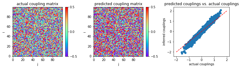
Large coupling variability \((g = 4)\)
Now, let us consider the regime of large coupling variability, \(g=4\) for instance.
In [12]:
g = 4.0
w0 = np.random.normal(0.0,g/np.sqrt(n),size=(n,n))

s = simulate.generate_data(w0,l)
Without our stopping criterion
When we do not apply our stopping criterion to MLE:
In [13]:
start_time = timeit.default_timer()

w = inference.mle(s,rate,stop_criterion='no')

stop_time=timeit.default_timer()
run_time=stop_time-start_time
print('run_time:',run_time)
('run_time:', 158.41191506385803)
In [14]:
plt.figure(figsize=(11,3.2))

plt.subplot2grid((1,3),(0,0))
plt.title('actual coupling matrix')
plt.imshow(w0,cmap='rainbow',origin='lower')
plt.xlabel('j')
plt.ylabel('i')
plt.clim(-0.5,0.5)
plt.colorbar(fraction=0.045, pad=0.05,ticks=[-0.5,0,0.5])

plt.subplot2grid((1,3),(0,1))
plt.title('predicted coupling matrix')
plt.imshow(w,cmap='rainbow',origin='lower')
plt.xlabel('j')
plt.ylabel('i')
plt.clim(-0.5,0.5)
plt.colorbar(fraction=0.045, pad=0.05,ticks=[-0.5,0,0.5])

plt.subplot2grid((1,3),(0,2))
plt.title('predicted couplings vs. actual couplings')
plt.plot([-2.0,2.0],[-2.0,2.0],'r--')
plt.scatter(w0,w)
plt.xlabel('actual couplings')
plt.ylabel('inferred couplings')

plt.tight_layout(h_pad=1, w_pad=1.5)
plt.show()
In [15]:
MSE = np.mean((w-w0)**2)
print('MSE:',MSE)
('MSE:', 0.01781885966000276)
With our stopping criterion
When our stopping criterion is applied to MLE:
In [16]:
start_time = timeit.default_timer()

w = inference.mle(s,rate,stop_criterion='yes')

stop_time=timeit.default_timer()
run_time=stop_time-start_time
print('run_time:',run_time)
('run_time:', 76.32810497283936)
In [17]:
plt.figure(figsize=(11,3.2))

plt.subplot2grid((1,3),(0,0))
plt.title('actual coupling matrix')
plt.imshow(w0,cmap='rainbow',origin='lower')
plt.xlabel('j')
plt.ylabel('i')
plt.clim(-0.5,0.5)
plt.colorbar(fraction=0.045, pad=0.05,ticks=[-0.5,0,0.5])

plt.subplot2grid((1,3),(0,1))
plt.title('predicted coupling matrix')
plt.imshow(w,cmap='rainbow',origin='lower')
plt.xlabel('j')
plt.ylabel('i')
plt.clim(-0.5,0.5)
plt.colorbar(fraction=0.045, pad=0.05,ticks=[-0.5,0,0.5])

plt.subplot2grid((1,3),(0,2))
plt.title('predicted couplings vs. actual couplings')
plt.plot([-2.0,2.0],[-2.0,2.0],'r--')
plt.scatter(w0,w)
plt.xlabel('actual couplings')
plt.ylabel('inferred couplings')

plt.tight_layout(h_pad=1, w_pad=1.5)
plt.show()
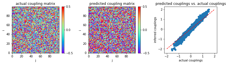
In [18]:
MSE = np.mean((w-w0)**2)
print('MSE:',MSE)
('MSE:', 0.0172333170396427)
As in the small coupling variability regime, our stopping criterion makes MLE slightly better (in accuracy) and significantly faster.