Thouless-Anderson-Palmer mean field approximation
![]()
We show in the following the performance of Thouless-Anderson-Palmer mean field approximation (TAP) in inferring couplings between variables from observed configurations. Similar to nMF, TAP works well only in the regime of large sample sizes and small coupling variability. However, this method leads to poor inference results in the regime of small sample sizes and/or large coupling variability.
As before, we import the packages to the jupyter notebook:
In [1]:
import numpy as np
import sys
import matplotlib.pyplot as plt
import simulate
import inference
%matplotlib inline

np.random.seed(1)
Small coupling variability \((g = 2)\) and small sample size \((L = 2 \times 10^3)\)
As with the other methods, we first use the same parameter setting: \(N = 100\), \(g = 2.0\), and \(L=2000\).
In [2]:
# parameter setting:
n = 100
g = 2.0
w0 = np.random.normal(0.0,g/np.sqrt(n),size=(n,n))
In [3]:
l = 2000
s = simulate.generate_data(w0,l)
We apply TAP to recover the coupling matrix w from variable
configurations s.
In [4]:
w = inference.tap(s)
We plot the heat map of inferred coupling matrix w and compare with
the actual couplings w0:
In [5]:
plt.figure(figsize=(11,3.2))

plt.subplot2grid((1,3),(0,0))
plt.title('actual coupling matrix')
plt.imshow(w0,cmap='rainbow',origin='lower')
plt.xlabel('j')
plt.ylabel('i')
plt.clim(-0.5,0.5)
plt.colorbar(fraction=0.045, pad=0.05,ticks=[-0.5,0,0.5])

plt.subplot2grid((1,3),(0,1))
plt.title('predicted coupling matrix')
plt.imshow(w,cmap='rainbow',origin='lower')
plt.xlabel('j')
plt.ylabel('i')
plt.clim(-0.5,0.5)
plt.colorbar(fraction=0.045, pad=0.05,ticks=[-0.5,0,0.5])

plt.subplot2grid((1,3),(0,2))
plt.title('predicted couplings vs. actual couplings')
plt.plot([-1,1],[-1,1],'r--')
plt.scatter(w0,w)
plt.xlabel('actual couplings')
plt.ylabel('inferred couplings')

plt.tight_layout(h_pad=1, w_pad=1.5)
plt.show()
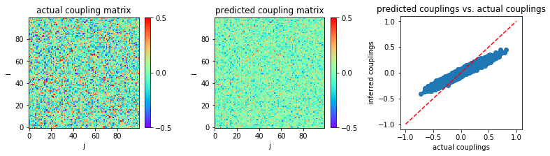
The mean square error between actual couplings and predicted couplings is calculated:
In [6]:
MSE = np.mean((w-w0)**2)
print('MSE:',MSE)
('MSE:', 0.009013103811623076)
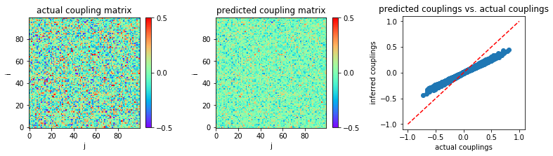
Small coupling variability \((g = 2)\) and large sample size \((L = 10^5)\)
Now, assume that we have a much larger number of samples, \(L=10^5\) for instance.
In [7]:
l = 100000
s = simulate.generate_data(w0,l)
In [8]:
w = inference.tap(s)
The inference result for this case is shown below:
In [9]:
plt.figure(figsize=(11,3.2))

plt.subplot2grid((1,3),(0,0))
plt.title('actual coupling matrix')
plt.imshow(w0,cmap='rainbow',origin='lower')
plt.xlabel('j')
plt.ylabel('i')
plt.clim(-0.5,0.5)
plt.colorbar(fraction=0.045, pad=0.05,ticks=[-0.5,0,0.5])

plt.subplot2grid((1,3),(0,1))
plt.title('predicted coupling matrix')
plt.imshow(w,cmap='rainbow',origin='lower')
plt.xlabel('j')
plt.ylabel('i')
plt.clim(-0.5,0.5)
plt.colorbar(fraction=0.045, pad=0.05,ticks=[-0.5,0,0.5])

plt.subplot2grid((1,3),(0,2))
plt.title('predicted couplings vs. actual couplings')
plt.plot([-1,1],[-1,1],'r--')
plt.scatter(w0,w)
plt.xlabel('actual couplings')
plt.ylabel('inferred couplings')

plt.tight_layout(h_pad=1, w_pad=1.5)
plt.show()
In [10]:
MSE = np.mean((w-w0)**2)
print('MSE:',MSE)
('MSE:', 0.008301534465467005)
The inference performance given by this method is still inaccurate, even for this larger number of samples.
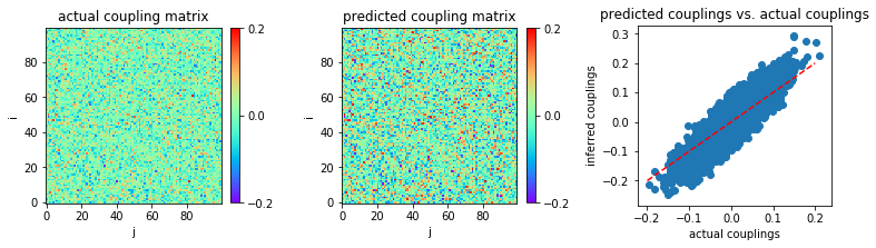
Very small coupling variability \((g = 0.5)\) and small sample size \((L = 2 \times 10^3)\)
Now, let us consider very small coupling variability, \(g = 0.5\) for instance.
In [11]:
g = 0.5
w0 = np.random.normal(0.0,g/np.sqrt(n),size=(n,n))
The data length \(L=2000\) is used as the first try.
In [12]:
l = 2000
s = simulate.generate_data(w0,l)
In [13]:
w = inference.tap(s)
In [14]:
plt.figure(figsize=(11,3.2))

plt.subplot2grid((1,3),(0,0))
plt.title('actual coupling matrix')
plt.imshow(w0,cmap='rainbow',origin='lower')
plt.xlabel('j')
plt.ylabel('i')
plt.clim(-0.2,0.2)
plt.colorbar(fraction=0.045, pad=0.05,ticks=[-0.2,0,0.2])

plt.subplot2grid((1,3),(0,1))
plt.title('predicted coupling matrix')
plt.imshow(w,cmap='rainbow',origin='lower')
plt.xlabel('j')
plt.ylabel('i')
plt.clim(-0.2,0.2)
plt.colorbar(fraction=0.045, pad=0.05,ticks=[-0.2,0,0.2])

plt.subplot2grid((1,3),(0,2))
plt.title('predicted couplings vs. actual couplings')
plt.plot([-0.2,0.2],[-0.2,0.2],'r--')
plt.scatter(w0,w)
plt.xlabel('actual couplings')
plt.ylabel('inferred couplings')

plt.tight_layout(h_pad=1, w_pad=1.5)
plt.show()
In [15]:
MSE = np.mean((w-w0)**2)
print('MSE:',MSE)
('MSE:', 0.0011565379679183974)
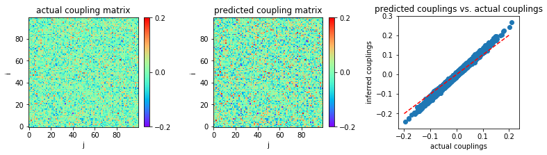
Very small coupling variability \((g = 0.5)\) and large sample size \((L = 10^5)\)
For a very large number of samples, \(L=10^5\):
In [16]:
l = 100000
s = simulate.generate_data(w0,l)
w = inference.tap(s)
In [17]:
plt.figure(figsize=(11,3.2))

plt.subplot2grid((1,3),(0,0))
plt.title('actual coupling matrix')
plt.imshow(w0,cmap='rainbow',origin='lower')
plt.xlabel('j')
plt.ylabel('i')
plt.clim(-0.2,0.2)
plt.colorbar(fraction=0.045, pad=0.05,ticks=[-0.2,0,0.2])

plt.subplot2grid((1,3),(0,1))
plt.title('predicted coupling matrix')
plt.imshow(w,cmap='rainbow',origin='lower')
plt.xlabel('j')
plt.ylabel('i')
plt.clim(-0.2,0.2)
plt.colorbar(fraction=0.045, pad=0.05,ticks=[-0.2,0,0.2])

plt.subplot2grid((1,3),(0,2))
plt.title('predicted couplings vs. actual couplings')
plt.plot([-0.2,0.2],[-0.2,0.2],'r--')
plt.scatter(w0,w)
plt.xlabel('actual couplings')
plt.ylabel('inferred couplings')

plt.tight_layout(h_pad=1, w_pad=1.5)
plt.show()
In [18]:
MSE = np.mean((w-w0)**2)
print('MSE:',MSE)
('MSE:', 0.00014564314455345025)
Similar to nMF, TAP works well only in the limit of large sample sizes and very small coupling variability.