Previous topic

Thouless-Anderson-Palmer mean field approximation

Next topic

Exact mean field approximation¶

Exact mean field (eMF) is another mean field approximation, similar to nMF and TAP. We show in the following that we can improve the performance of this method by adding our stopping criterion. In general, eMF outperforms nMF and TAP, but it is still worse than FEM and MLE, especially in the limit of small sample sizes and large coupling variability.

In [1]:

import numpy as np
import sys
import matplotlib.pyplot as plt
import simulate
import inference
%matplotlib inline

np.random.seed(1)

Small coupling variability $(g = 2)$ and small sample size $(L = 2 \times 10^3)$¶

As with comparisons with other methods, we first use the same parameter setting: $N = 100$, $g = 2.0$, and $L=2000$.

In [2]:

# parameter setting:
n = 100
g = 2.0
w0 = np.random.normal(0.0,g/np.sqrt(n),size=(n,n))

In [3]:

l = 2000
s = simulate.generate_data(w0,l)

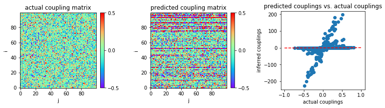
Unlike nMF and TAP, eMF is an iterative method. We first apply this method as described in the literature, without a stopping criterion. As expected, it overfits in the limit of small sample sizes.

In [4]:

w = inference.emf(s,stop_criterion='no')

In [5]:

plt.figure(figsize=(11,3.2))

plt.subplot2grid((1,3),(0,0))
plt.title('actual coupling matrix')
plt.imshow(w0,cmap='rainbow',origin='lower')
plt.xlabel('j')
plt.ylabel('i')
plt.clim(-0.5,0.5)
plt.colorbar(fraction=0.045, pad=0.05,ticks=[-0.5,0,0.5])

plt.subplot2grid((1,3),(0,1))
plt.title('predicted coupling matrix')
plt.imshow(w,cmap='rainbow',origin='lower')
plt.xlabel('j')
plt.ylabel('i')
plt.clim(-0.5,0.5)
plt.colorbar(fraction=0.045, pad=0.05,ticks=[-0.5,0,0.5])

plt.subplot2grid((1,3),(0,2))
plt.title('predicted couplings vs. actual couplings')
plt.plot([-1,1],[-1,1],'r--')
plt.scatter(w0,w)
plt.xlabel('actual couplings')
plt.ylabel('inferred couplings')

plt.tight_layout(h_pad=1, w_pad=1.5)
plt.show()

In [6]:

MSE = np.mean((w-w0)**2)
print('MSE:',MSE)

('MSE:', 94.26756796949678)

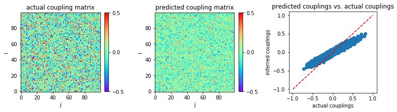
Now, we apply our stopping criterion with eMF. According to this criterion, we stop the iteration when the discrepancy starts to increase. This option is selected by setting stop_criterion='yes'. We will see that the eMF performance is significantly improved.

In [7]:

w = inference.emf(s,stop_criterion='yes')

The inference result is shown:

In [8]:

plt.figure(figsize=(11,3.2))

plt.subplot2grid((1,3),(0,0))
plt.title('actual coupling matrix')
plt.imshow(w0,cmap='rainbow',origin='lower')
plt.xlabel('j')
plt.ylabel('i')
plt.clim(-0.5,0.5)
plt.colorbar(fraction=0.045, pad=0.05,ticks=[-0.5,0,0.5])

plt.subplot2grid((1,3),(0,1))
plt.title('predicted coupling matrix')
plt.imshow(w,cmap='rainbow',origin='lower')
plt.xlabel('j')
plt.ylabel('i')
plt.clim(-0.5,0.5)
plt.colorbar(fraction=0.045, pad=0.05,ticks=[-0.5,0,0.5])

plt.subplot2grid((1,3),(0,2))
plt.title('predicted couplings vs. actual couplings')
plt.plot([-1,1],[-1,1],'r--')
plt.scatter(w0,w)
plt.xlabel('actual couplings')
plt.ylabel('inferred couplings')

plt.tight_layout(h_pad=1, w_pad=1.5)
plt.show()

In [9]:

MSE = np.mean((w-w0)**2)
print('MSE:',MSE)

('MSE:', 0.0072491113790595)

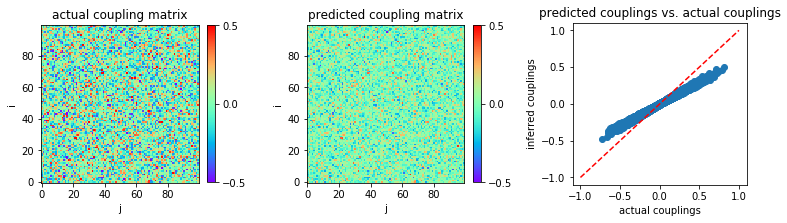
Small coupling variability $(g = 2)$ and large sample size $(L = 10^5)$¶

Now, let consider the large sample size regime, $L = 100000$ for instance.

In [10]:

l = 100000
s = simulate.generate_data(w0,l)

In [11]:

w = inference.emf(s,stop_criterion='yes')

The inference result is shown:

In [12]:

plt.figure(figsize=(11,3.2))

plt.subplot2grid((1,3),(0,0))
plt.title('actual coupling matrix')
plt.imshow(w0,cmap='rainbow',origin='lower')
plt.xlabel('j')
plt.ylabel('i')
plt.clim(-0.5,0.5)
plt.colorbar(fraction=0.045, pad=0.05,ticks=[-0.5,0,0.5])

plt.subplot2grid((1,3),(0,1))
plt.title('predicted coupling matrix')
plt.imshow(w,cmap='rainbow',origin='lower')
plt.xlabel('j')
plt.ylabel('i')
plt.clim(-0.5,0.5)
plt.colorbar(fraction=0.045, pad=0.05,ticks=[-0.5,0,0.5])

plt.subplot2grid((1,3),(0,2))
plt.title('predicted couplings vs. actual couplings')
plt.plot([-1,1],[-1,1],'r--')
plt.scatter(w0,w)
plt.xlabel('actual couplings')
plt.ylabel('inferred couplings')

plt.tight_layout(h_pad=1, w_pad=1.5)
plt.show()

In [13]:

MSE = np.mean((w-w0)**2)
print('MSE:',MSE)

('MSE:', 0.006379354359631724)

From the above result, we conclude that eMF works better than eMF and TAP but not as well as FEM and MLE.

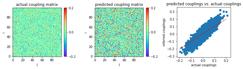
Very small coupling variability $(g = 0.5)$ and small sample size $(L = 2 \times 10^3)$¶

Now, let us consider a regime of very small coupling variability, $g = 0.5$.

In [14]:

g = 0.5
w0 = np.random.normal(0.0,g/np.sqrt(n),size=(n,n))

We use a data length $L = 2000$ for the first example in this regime.

In [15]:

l = 2000
s = simulate.generate_data(w0,l)

In [16]:

w = inference.emf(s,stop_criterion='yes')

In [17]:

plt.figure(figsize=(11,3.2))

plt.subplot2grid((1,3),(0,0))
plt.title('actual coupling matrix')
plt.imshow(w0,cmap='rainbow',origin='lower')
plt.xlabel('j')
plt.ylabel('i')
plt.clim(-0.2,0.2)
plt.colorbar(fraction=0.045, pad=0.05,ticks=[-0.2,0,0.2])

plt.subplot2grid((1,3),(0,1))
plt.title('predicted coupling matrix')
plt.imshow(w,cmap='rainbow',origin='lower')
plt.xlabel('j')
plt.ylabel('i')
plt.clim(-0.2,0.2)
plt.colorbar(fraction=0.045, pad=0.05,ticks=[-0.2,0,0.2])

plt.subplot2grid((1,3),(0,2))
plt.title('predicted couplings vs. actual couplings')
plt.plot([-0.2,0.2],[-0.2,0.2],'r--')
plt.scatter(w0,w)
plt.xlabel('actual couplings')
plt.ylabel('inferred couplings')

plt.tight_layout(h_pad=1, w_pad=1.5)
plt.show()

In [18]:

MSE = np.mean((w-w0)**2)
print('MSE:',MSE)

('MSE:', 0.001573704964233979)

Very small coupling variability $(g = 0.5)$ and large sample size $(L = 10^5)$¶

Consider now a much larger sample size, $L = 10^5.$

In [19]:

l = 100000
s = simulate.generate_data(w0,l)

In [20]:

w = inference.emf(s,stop_criterion='yes')

In [21]:

plt.figure(figsize=(11,3.2))

plt.subplot2grid((1,3),(0,0))
plt.title('actual coupling matrix')
plt.imshow(w0,cmap='rainbow',origin='lower')
plt.xlabel('j')
plt.ylabel('i')
plt.clim(-0.2,0.2)
plt.colorbar(fraction=0.045, pad=0.05,ticks=[-0.2,0,0.2])

plt.subplot2grid((1,3),(0,1))
plt.title('predicted coupling matrix')
plt.imshow(w,cmap='rainbow',origin='lower')
plt.xlabel('j')
plt.ylabel('i')
plt.clim(-0.2,0.2)
plt.colorbar(fraction=0.045, pad=0.05,ticks=[-0.2,0,0.2])

plt.subplot2grid((1,3),(0,2))
plt.title('predicted couplings vs. actual couplings')
plt.plot([-0.2,0.2],[-0.2,0.2],'r--')
plt.scatter(w0,w)
plt.xlabel('actual couplings')
plt.ylabel('inferred couplings')

plt.tight_layout(h_pad=1, w_pad=1.5)
plt.show()

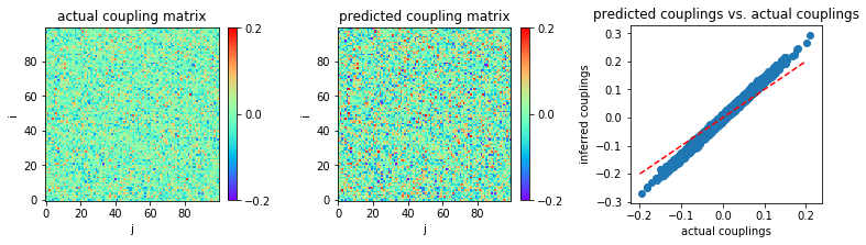
In [22]:

MSE = np.mean((w-w0)**2)
print('MSE:',MSE)

('MSE:', 0.0003542442179127955)

As with other mean field approximations such as nMF and TAP, eMF works well only in the limit of large sample sizes and very small coupling variability.

Previous topic

Next topic

Exact mean field approximation¶

Small coupling variability \((g = 2)\) and small sample size \((L = 2 \times 10^3)\)¶

Small coupling variability \((g = 2)\) and large sample size \((L = 10^5)\)¶

Very small coupling variability \((g = 0.5)\) and small sample size \((L = 2 \times 10^3)\)¶

Very small coupling variability \((g = 0.5)\) and large sample size \((L = 10^5)\)¶

Previous topic

Next topic

Quick search

Exact mean field approximation¶

Small coupling variability \((g = 2)\) and small sample size \((L = 2 \times 10^3)\)¶

Small coupling variability \((g = 2)\) and large sample size \((L = 10^5)\)¶

Very small coupling variability \((g = 0.5)\) and small sample size \((L = 2 \times 10^3)\)¶

Very small coupling variability \((g = 0.5)\) and large sample size \((L = 10^5)\)¶